Market Earth: the law of motion for capital accumulation: ramsey's way

Thursday, February 14, 2013

the law of motion for capital accumulation: ramsey's way

$\dot{k}=f(k) - \delta\,k - c$

"where k is capital per worker, $\dot{k}$ is change in capital per worker over time, c is consumption per worker, f(k) is output per worker, and $\delta\,$ is the depreciation rate of capital. This equation simply states that investment, or increase in capital per worker is that part of output which is not consumed, minus the rate of depreciation of capital. Investment is, therefore, the same as savings.

$I=sY$

where I is the level of investment, Y is level of income and s is the savings rate, or the proportion of income that is saved.
The second equation concerns the saving behavior of households and is less intuitive. If households are maximizing their consumption intertemporally, at each point in time they equate the marginal benefit of consumption today with that of consumption in the future, or equivalently, the marginal benefit of consumption in the future with its marginal cost. Because this is an intertemporal problem this means an equalization of rates rather than levels. There are two reasons why households prefer to consume now rather than in the future. First, they discount future consumption. Second, because the utility function is concave, households prefer a smooth consumption path. An increasing or a decreasing consumption path lowers the utility of consumption in the future. Hence the following relationship characterizes the optimal relationship between the various rates:
rate of return on savings = rate at which consumption is discounted − percent change in marginal utility times the growth of consumption.
Mathematically:

$r = \rho\ - %dMU*\dot c \,$

A class of utility functions which are consistent with a steady state of this model are the isoelastic or constant relative risk aversion (CRRA) utility functions, given by:

$u(c) = \frac{c^{1-\theta}-1} {1-\theta} \,$

In this case we have:

$%dMU = \frac{\frac{d^2u}{dc^2}}{\frac{du}{dc}} = -\frac{\theta}{c}$

Then solving the above dynamic equation for consumption growth we get:

$\frac{\dot c} {c} = \frac{r - \rho} {\theta} \,$

which is the second key dynamic equation of the model and is usually called the "Euler equation".
With a neoclassical production function with constant returns to scale, the interest rate, r, will equal the marginal product of capital per worker. One particular case is given by the Cobb–Douglas production function

$y=k^\alpha \,$

which implies that the gross interest rate is

$R = \alpha k^{\alpha-1} \,$

hence the net interest rate r

$r = R - \delta = \alpha k^{\alpha-1} - \delta \,$

Setting $\dot k$ and $\dot c$ equal to zero we can find the steady"

Ramsey, Frank P. (1928). "A Mathematical Theory of Saving". Economic Journal 38 (152): 543–559. JSTOR 2224098

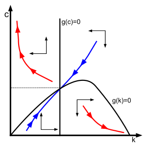
"Phase space graph (or phase diagram) of the Ramsey model. The blue line represents the dynamic adjustment (or saddle) path of the economy in which all the constraints present in the model are satisfied. It is a stable path of the dynamic system. The red lines represent dynamic paths which are ruled out by the transversality condition"

very much the perfect clark kent no ?